An SQL text by Erland Sommarskog, SQL Server
MVP. Most recent update 2026-10-17.
Copyright applies to this text. See here for font conventions used in this article.
This short story covers two different optimization features in SQL Server: String summary statistics and row goals. The latter is something that some readers may have heard of, whereas I suspect that fewer readers are acquainted with string summary statistics, despite that they have been in the product for a long time (as have row goals). The reason I'm bringing them together in one article is that this story is based on a real-world case that we discussed on an internal forum where we Data Platform MVPs can interact with each other as well as with persons from the product group. It started with Rudi Bruchez asking for help with speeding up a query, whereupon Hugo Kornelis, Simon Sabin and myself jumped in. The discussion led to Simon composing a repro which produced results that left us completely baffled until Vassilis Papadimos from the optimizer team set us straight. I felt that the lessons of this internal discussion could be of general interest, so I decided to share our learnings – with the consent of the others – by writing this article.
While the title has string summary statistics first, and they are sort of "the star of the show", we will start with row goals, as that comes naturally with Rudi's problem. After that we turn to the string summary statistics. In the concluding chapter, I will come back to Rudi's problem for some final observations.
Table of Contents
Row_number vs. TOP and OFFSET FETCH
String Summary Statistics and the Legacy Cardinality Estimator
Some of the demos in this article run in the Northgale database. This is an inflated version of the very old demo database Northwind. To install Northgale, first run Northwind.sql and then Northgale.sql which uses the data in Northwind. I use Northgale in several of my articles and presentations, but I often tweak it for the particular topic at hand, so there are some minor variations (which I can't keep track of myself :-). Therefore, if you already have Northgale, make a new download, so that the results will agree with what I'm saying in the article.
Northwind always installs itself in the same folder as where you have the master database, whereas the script for Northgale respects your default settings for data and log directories. Northwind is less than 10 MB in size and has 830 orders, whereas Northgale takes up 1.3 GB and has a little more than one million orders. (You will need 4 GB extra to build the database for a secondary log file which is dropped once the script completes.)
Beside installing the database, I also recommend you to run
EXEC sp_configure 'cost threshold for parallelism', 5
RECONFIGURE
This is the default setting for this configuration parameter, but many consider it to be best practice to set it to a higher value like 30 or 50, and you might have done that. However, the outcome of the demos may not agree with what I say in the article with the threshold set to a higher value. (I'm here assuming that you are running the demos on a private instance on your laptop or similar. If you are running the demos on a shared instance, by all means, do not change the configuration as it could affect other users.)
Rant: As for this being best practice... The common argument is that the default comes from a time when hardware was completely different from today. But I don't think I've ever seen any real "scientific" proof that you get better performance by raising the threshold, and I can't escape the feeling that this is just a fad that has caught on. Then again, I certainly do not have any evidence that the default of 5 is better. Common sense tells me that on a busy OLTP system with many users, it can definitely make sense to raise the limit, because you don't want queries to monopolise the CPU by going parallel. On the other hand, on a system with lots of cores where a handful of business analysts run vile queries, raising the threshold may very well be a go-slower button.
Rudi encountered his problem on SQL 2022. However, I have only tested the queries in this article on SQL 2025 with compatibility level 170 (unless otherwise noted). Thus, if you are running on older version or lower compatibility level, you may see different results.
The purpose of this section is not to provide a complete discussion about row goals, but to discuss situations where row goals work less well and affect your performance negatively. For this reason, I will simplify the discussion a little bit. For an in-depth discussion about row goals as such, please see Paul White's articles Inside the Optimizer: Row Goals In Depth and Setting and Identifying Row Goals in Execution Plan (which I consulted myself, before I started writing this chapter).
In Rudi's starting post, he had this query (anonymised from the source system):
WITH cte AS
   (SELECT ...,
    ROW_NUMBER() OVER(ORDER BY [T0].[Id] ASC) AS SYSROWNUMBER
    FROM Item T0
    LEFT OUTER JOIN Unit T1 ON T0.fk = T1.pk
    WHERE T0.[ActiveState] = 0
    AND T0.ModifiedDate > DATEFROMPARTS(2022, 12, 31)
    AND (T0.varchar1 LIKE 'something%' ESCAPE '\'
            COLLATE SQL_Latin1_General_CP1_CI_AI
         OR T0.varchar2 LIKE '%something%' ESCAPE '\'
            COLLATE SQL_Latin1_General_CP1_CI_AI)
)
SELECT *
FROM cte
WHERE [SYSROWNUMBER] >= 1 AND [SYSROWNUMBER] <= 200
The purpose is to retrieve data from two tables based on some criteria and then present the data in a paged fashion, this being the query for the first page. You may be a little bewildered by those ESCAPE and COLLATE clauses. For this chapter, we will largely ignore them, but we will come to the effect of them later.
This query was emitted by the client, and it was beyond Rudi's control to change it. What he could do was to add indexes and Query Store hints. With Query Store hints you can inject query hints, for instance to control MAXDOP, into a query without touching the text. For more details, see the topic Query Store Hints in Microsoft Learn.
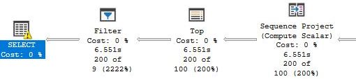
As the discussion progressed, Rudi also shared the execution plan for the query with us (to keep the page width in check, I've split up the image over two lines):
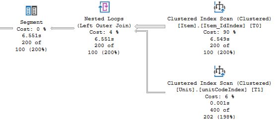
The overall shape of the plan is reasonable. According to Rudi, most of the rows have ActiveState = 0, so that condition is not selective. The filter on ModifiedDate singles out a little more than two years of data (Rudi posted his question at the end of April 2025), so neither that condition is likely to be selective enough to make it meaningful to use any index on that column. The conditions on varchar1 and varchar2 cannot use indexes because the columns are entangled in an expression (i.e. the COLLATE clauses). Add to this that the search pattern for varchar2 has a leading wildcard. When it comes to the table Unit in the lower Clustered Index Scan operator, that table only has two rows, so that scan is nothing to worry about.
Note: The reader may note that the COLLATE clauses are applied on the search strings and not the columns themselves. However, when you add a COLLATE clause on one side in an expression, it propagates to the other side as well, so the columns are indeed affected. For a more detailed discussion, see the topic Collation Precedence in Microsoft Learn.
Rudi's concern was not with the plan as such, but with the estimated costs for the Clustered Index Scan operator on the upper table, Item. In the XML he found these values:
<RelOp AvgRowSize="266" EstimateCPU="1.0725" EstimateIO="532.816"
EstimateRebinds="0" EstimateRewinds="0" EstimatedExecutionMode="Row"
EstimateRows="100" EstimateRowsWithoutRowGoal="329146"
EstimatedRowsRead="974858" LogicalOp="Clustered Index Scan" NodeId="6"
Parallel="false" PhysicalOp="Clustered Index Scan"
EstimatedTotalSubtreeCost="0.164939" TableCardinality="974858">
What particularly confused him was that the total cost for the node was 0.16, when the sum of EstimateCPU+EstimateIO was so much higher. The subtree cost was also the core of his concern, because he had concluded that parallelism would be the best way to speed up the query. But with that low estimate for the cost, the optimizer was utterly uninterested in parallelism.
Before I move on, a note about the size of the Item table. The value for TableCardinality is just below one million, and you may think that this is a relatively small table. However, the rows are apparently very wide. The execution-plan XML revealed that the execution of the CI Scan required over 712 000 logical reads, almost 6 GB of data. (Don't be confused by AvgRowSize being reported as 266. That is the size of the rows returned from the operator; it is not the size of the rows being read.)
Hugo Kornelis was the first to respond, and he identified that the low cost was due to the presence of a row goal. In the data above, there are two tokens of a row goal being present. One is the appearance of the attribute EstimateRowsWithoutRowGoal. The other token is exactly that EstimatedTotalSubtreeCost is not equal to EstimateCPU+EstimateIO. I learnt from Paul White's first article that row goals are an add-on to the normal optimisation process and they only adjust the total cost (which is what matters in the end), but the components that build up the original cost value are not adjusted.
So what is a row goal? As noted, Rudi's query asks for the first 200 rows by Id (the clustered index of Item). Without this filter on the row_number function, SQL Server would have to read Item from start to end to find all matching rows. But with this filter present, SQL Server can stop the scan as soon as 200 rows have been found. The optimizer realises that this reduces the cost of the operators to the right of the Top operator, and particularly the cost of the expensive one: the Clustered Index Scan on Item. This limit of the number of rows needed, 200 in this case, is known as a row goal. Although, the row goal the optimizer uses in this query is 100 rows, which is testified by the fact that it says 200 of 100 below the Top operator in the plan. (200 is the actual number of rows returned, 100 is the estimated number.) This is due to an imperfection that I will return to. For the discussion in this chapter, 100 or 200 is of little importance.
Row goals often appear with the TOP operator, OFFSET FETCH, as well as with filtering on row_number as in this example and a few more situations that Paul discusses in his article. Overall, row goals serve to make the optimizer better, since they reduce the estimated cost for a query that only returns a small portion of a larger number of rows. This can prevent parallelism being applied when there is no need to, and it can lead to a different plan shape than if no row goal had been present. For instance, compare the execution plan for this query in Northgale with the TOP clause commented out and activated:
DROP TABLE IF EXISTS #temp
SELECT -- TOP (100)
       O.OrderID, O.CustomerID, O.OrderDate, OD.ProductID, OD.Quantity
INTO   #temp
FROM   Orders O
JOIN   [Order Details] OD ON O.OrderID = OD.OrderID
Note: The purpose of the temp table is to avoid filling the grid in SSMS with lots of uninteresting rows. We will use this technique more than once in this article.
Without TOP, the query uses parallelism and the join is implemented with a Hash Join. With TOP, there is no parallelism, and the join is a Nested Loops Join.
However, as with most optimizer features, there are situations where row goals work against you, and Rudi's query is such an example. In this case, the optimizer estimates that the query before the filtering on row_number matches 329 146 rows (i.e. EstimateRowsWithoutRowGoal). That's about one third of the table. The optimizer has very little idea where in the table these rows are located, so it makes the naïve assumption that the matching rows are distributed evenly over the table. Therefore, the optimizer arrives at an estimate that the Scan operator only has to sift through around 300 rows before it can stop, and the optimizer scales down the overall cost accordingly. (300 rows, because the row goal is 100, and it thinks that around one third of the rows match.)
Looking at Rudi's query, does it seem that this assumption is correct? That depends on the nature of the Id column. Assume that it is a random GUID. Yes, in that case, there is no reason to assume any correlation between the values of Id and the values of the other filter columns. But assume instead that Id is a numeric surrogate key that grows monotonically, a very common situation. In this case, we can expect a very high degree of correlation between the columns Id and ModifiedDate. I don't know how far back in time the data in the table goes, but say that there is data for ten years. This means that to find the first matching rows, SQL Server will have to trawl through data for seven years or so, before finding the first match. That is, the better part of the table. And, thus, the cost that the optimizer arrived at after applying the row goal was a gross underestimation.
To study this situation a little more closely, let's look at a query in Northgale, which is drawn from Rudi's query:
DROP TABLE IF EXISTS #temp
SET STATISTICS TIME ON
; WITH CTE AS (
   SELECT O.OrderID, O.OrderDate, O.CustomerID, C.CustomerName,
          E.FirstName, E.LastName, P.ProductName, OD.Quantity, OD.UnitPrice,
          row_number() OVER(ORDER BY O.OrderID) AS rowno
   FROM   Orders O
   JOIN   "Order Details" OD ON O.OrderID = OD.OrderID
   JOIN   Customers C ON C.CustomerID = O.CustomerID
   JOIN   Employees E ON E.EmployeeID = O.EmployeeID
   JOIN   Products P ON P.ProductID = OD.ProductID
   WHERE  O.RequiredDate >= '20011201'
)
SELECT OrderID, OrderDate, CustomerID, CustomerName,
       FirstName, LastName, ProductName, Quantity, UnitPrice
INTO   #temp
FROM   CTE
WHERE  rowno BETWEEN 1 AND 200
SET STATISTICS TIME OFF
A couple of points about this query and the data in Northgale.
I run this twice, discarding the first execution to know that I am reading the data from the cache. When I run it without display of execution plan, I get something like this:
SQL Server Execution Times:
CPU time = 250 ms, elapsed time = 254 ms.
If you enable display of the execution plan, you will find that the plan resembles the plan for Rudi's query, even if there are a number of Nested Loops operators due to the extra tables.
If we dive into the XML and look at the RelOp node for the Clustered Index Scan, we find this:
<RelOp AvgRowSize="31" EstimateCPU="1.13547" EstimateIO="18.4868"
EstimateRebinds="0" EstimateRewinds="0" EstimatedExecutionMode="Row"
EstimateRows="14.8388" EstimateRowsWithoutRowGoal="122419"
EstimatedRowsRead="120.185" LogicalOp="Clustered Index Scan" NodeId="13"
Parallel="false" PhysicalOp="Clustered Index Scan"
EstimatedTotalSubtreeCost="0.00564218" TableCardinality="1032100">
The exact values may vary a little between your machine and mine.
Note: Rather than looking into the XML, you can also click the operator in the diagram and select Properties from the context menu. I decided to show the XML to align with what I had for Rudi's query above. Note that the popup is less useful here, because it does not include EstimateRowsWithoutRowGoal.
This is reminiscent of what we saw above with Rudi's query. Particularly, since we see the presence of EstimateRowsWithoutRowGoal and that the estimated subtree cost is much lower than the sum of the estimated CPU and IO costs, we can tell that a row goal is present. The reason the cost is so low is that the optimizer looks in the statistics histogram for RequiredDate and finds that there are around 120 000 qualifying rows. To verify this, you can run this query, which I refrain from explaining in the interest of brevity:
DECLARE @statsid int
SELECT @statsid = sc.stats_id
FROM   sys.stats_columns sc
JOIN   sys.columns c ON c.object_id = sc.object_id
                    AND c.column_id = sc.column_id
WHERE  sc.object_id = object_id('dbo.Orders')
  AND  sc.stats_column_id = 1
  AND  c.name = 'RequiredDate'

SELECT SUM(range_rows + equal_rows)
FROM   sys.dm_db_stats_histogram(object_id('dbo.Orders'), @statsid)
WHERE  range_high_key > convert(sql_variant, convert(date, '2001-12-01'))
The example query asks for 200 rows. The optimizer estimates that it has to read around 15 orders to get 200 rows in total for the query. (As each row in Orders matches a couple of rows in Order Details.) The optimizer has no information of how the matching rows are distributed, so it makes its regular assumption about a uniform distribution and thinks that 15 rows will pop up early in the scan, and therefore it scales cost drastically. But those 120 000 rows out of a little more than one million are all located at the end of the clustered index, so SQL Server has to work a lot harder to find those 15 rows.
Say now that we have identified that the row goal works against us, and we want to improve performance by adding parallelism. Can we do that? Yes, there is a hint to disable the row goal:
DROP TABLE IF EXISTS #temp
SET STATISTICS TIME ON
; WITH CTE AS (
   SELECT O.OrderID, O.OrderDate, O.CustomerID, C.CustomerName,
          E.FirstName, E.LastName, P.ProductName, OD.Quantity, OD.UnitPrice,
          row_number() OVER(ORDER BY O.OrderID) AS rowno
   FROM   Orders O
   JOIN   "Order Details" OD ON O.OrderID = OD.OrderID
   JOIN   Customers C ON C.CustomerID = O.CustomerID
   JOIN   Employees E ON E.EmployeeID = O.EmployeeID
   JOIN   Products P ON P.ProductID = OD.ProductID
   WHERE  O.RequiredDate >= '20011201'
)
SELECT OrderID, OrderDate, CustomerID, CustomerName,
       FirstName, LastName, ProductName, Quantity, UnitPrice
INTO   #temp
FROM   CTE
WHERE  rowno BETWEEN 1 AND 200
OPTION (USE HINT('DISABLE_OPTIMIZER_ROWGOAL'))
SET STATISTICS TIME OFF
When I run this on my machine, I get:
SQL Server Execution Times:
CPU time = 843 ms, elapsed time = 108 ms.
Success, it runs faster! Well, the DBA may disagree. The query now runs faster for the user, thanks to parallelism, but it takes more CPU resources.
I should point out that you may see a different outcome, as there are a few it depends here. One is how many CPU cores that are available and the setting of the configuration parameters max degree of parallelism (which also can be set as a database-scoped configuration) and cost threshold for parallelism. Furthermore, the edition of SQL Server matters. I ran the above on an instance where I have Enterprise Developer Edition, and the plan I got when I added the hint includes operators in batch mode, an Enterprise-only feature. I also tested the query on an instance with Standard Developer Edition. In this case, I got a non-parallel plan. Nevertheless, I still got a performance improvement, if somewhat smaller.
When you are working with a query where there is a row goal, you may ask yourself: How do I know if there is a menacing correlation? The quick answer is that you may know your data. But if you are asked to look at a query in a database you are not familiar with, the correlation may be less apparent to you. In this case, the execution plan may offer useful information. If we look at the properties for the CI Scan operator for our example query, there is a very strong indication when we compare the number of actual number of rows read with the estimated:

The optimizer estimated that it would have to read 120 rows to find those 15 orders with RequiredDate in December 2001 or later, but it actually had to read over 900 000 orders. I would say that this is quite a sure sign of a row goal going bad because of a correlation between the filter conditions and the ordering criteria for the row goal. But, as always, differences between actual and estimated numbers can also be due to the regular culprits: outdated statistics, applying of default estimates etc. We will see an example of the latter in the next chapter.
Unfortunately, though, this comparison is only possible on SQL 2025 or later. If you go back and look at the XML snippet from Rudi's case, which was from SQL 2022, you will see that EstimatedRowsRead is equal to the table cardinality. As Hugo Kornelis explained to me, up to SQL 2022, EstimateRowsRead was the number of rows that the optimizer estimated that SQL Server would have to read if there had not been any row goal at all. It is a little confusing with all these different EstimateRowsXXX, but EstimateRows and EstimateRowsWithoutRowGoal relates to how many rows the operator returns, whereas EstimateRowsRead is about how many rows SQL Server will need to read in total to find these rows. And obviously, for a Clustered Index Scan operator, this will be all rows in the table where there is no row goal. But when there is a row goal, it is certainly more interesting to know how many rows the optimizer thinks that it actually has to read, and therefore Microsoft made this change in SQL 2025.
Before we leave row goals, I'd like to show a case where a row goal leads to very bad performance. This is drawn from something I ran into a couple of years ago and it did not make me very happy. We will start nice and easy, though. Run this script to add one more order for each employee, later than any of the other orders:
INSERT Orders(OrderID, CustomerID, EmployeeID, OrderDate, RequiredDate, ShippedDate,
              ShipVia, Freight,ShipName, ShipAddress, ShipCity, ShipPostalCode,
              ShipCountry, Discount, TotalAmount, Status)
   SELECT 2000000 + EmployeeID, 'RATTC', EmployeeID, '20030101', '20030101', '20030101',
          2048, 10, 'Nisse Nils', 'Nilsgatan 11', 'Nilsstad', '80808',
          'Sweden', 0, 200, 'N'
   FROM   Employees
Now we run a query to retrieve data about the most recent order for each employee. We run it in two fashions, without and with an index hint. To compare the executions, we flush the cache before the executions (for this reason it is not advisable to run this on an instance you are sharing with other users):
DROP TABLE IF EXISTS #temp1, #temp2
DBCC DROPCLEANBUFFERS
go
SET STATISTICS TIME ON
SELECT E.EmployeeID, E.FirstName, E.LastName,
       O.OrderID, O.OrderDate, O.Status, O.CustomerID
INTO   #temp1
FROM   Employees E
CROSS  APPLY (SELECT TOP (1) O.OrderID, O.OrderDate, O.Status, O.CustomerID
              FROM   Orders O
              WHERE  E.EmployeeID = O.EmployeeID
              ORDER  BY O.OrderID DESC) AS O
--OPTION (USE HINT('DISABLE_OPTIMIZER_ROWGOAL'))
SET STATISTICS TIME OFF
go
DBCC DROPCLEANBUFFERS
go
SET STATISTICS TIME ON
SELECT E.EmployeeID, E.FirstName, E.LastName,
       O.OrderID, O.OrderDate, O.Status, O.CustomerID
INTO   #temp2
FROM   Employees E
CROSS  APPLY (SELECT TOP (1) O.OrderID, O.OrderDate, O.Status, O.CustomerID
              FROM   Orders O WITH (INDEX = empid_ix)
              WHERE  E.EmployeeID = O.EmployeeID
              ORDER  BY O.OrderID DESC) AS O
SET STATISTICS TIME OFF
go
The plan for the first query, the one without the hint, looks like this:
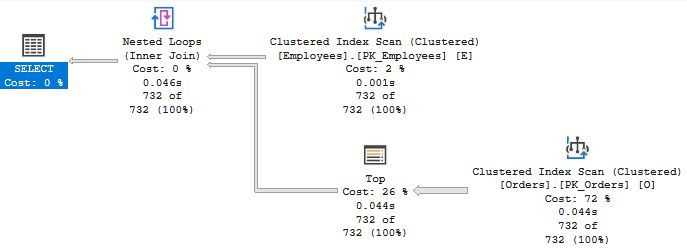
As you may suspect, the Top operator defines a row goal, which you can verify by looking at the properties for the Clustered Index Scan on Orders. The optimizer discards the use of the non-clustered index on EmployeeID, thinking If I use that index, I must do key lookups. I hate key lookups! Key lookups are expensive. And anyway, I should be able to quickly find a row for an employee by scanning just a few rows in the Orders table.
And, indeed, we have just set up data perfectly for the optimizer. It can't be any better. Yet, this is the outcome:
SQL Server Execution Times:
CPU time = 141 ms, elapsed time = 193 ms.
SQL Server Execution Times:
CPU time = 16 ms, elapsed time = 46 ms.
The version with the index hint outperforms the optimizer's idea. But to be fair: The costing model is based on yesterday's hardware with spinning disks where random I/O was a lot slower than on SSDs.
As I said, this was a very good setup for the optimizer's plan. Even with original data, the situation is not too unblessed. There are some employees with only a handful of orders, but even they have their latest order by the end of December 2001. In the real world, there may be employees who have been on extended leave. Or those who quit years ago. In the situation I ran into it was even worse. It was more like the situation after this UPDATE:
UPDATE Orders
SET    EmployeeID += 1
FROM   Orders O
WHERE  O.EmployeeID % 2 = 0
  AND  EXISTS (SELECT *
               FROM   Employees E
               WHERE  E.EmployeeID = O.EmployeeID + 1)

ALTER INDEX empid_ix ON Orders REBUILD
That is, about half of the employees do not have any orders at all. (Could be new recruits that joined the company just the other day.) Run the queries again. The plans do not change (keep in mind that since we rebuilt the index, the current plans are flushed from the cache), but the execution certainly takes longer time now:
SQL Server Execution Times:
CPU time = 19188 ms, elapsed time = 19277 ms.
SQL Server Execution Times:
CPU time = 16 ms, elapsed time = 65 ms.
In the previous example with RequiredDate, the optimizer had an excuse: It has absolutely no information about the correlation between RequiredDate and OrderID. But it is different this time. It has the cardinality for the Employees table. It has the density for Orders.EmployeeID which suggests that a lot of employees do not have any orders at all. Thus, it should realise that the scan will run through the entire table for many employees. But the optimizer is not smart enough to piece these data points together. If it at least had contemplated the risk of that plan and computed the cost for the worst case. But, no, if you hate key lookups, you hate key lookups and you avoid them like the plague. Even if that means you have to scan a million-row table again and again.
Anyway, uncomment the hint to disable the goal and run again:
SQL Server Execution Times:
CPU time = 1453 ms, elapsed time = 1429 ms.
Certainly better, but it still shuns the index and introduces an Index Spool. However, that is actually a correct decision! To wit, the plan for the query with the index hint also sports a row goal, and if you disable row goals for that query as well, you find that it runs slower than the query without the index hint.
So a lesson of this is that when a row goal works against you, the hint DISABLE_OPTIMIZER_ROWGOAL is not always the best solution to the problem. In this example, the row goal was after all on our side. But only with the use of the right index.
In our discussions around Rudi's problem, Simon Sabin composed a repro script (or a POC as he called it). I have taken his script and adapted it to cover the things I want to discuss in this chapter. Here is a definition of the table we will work with and an INSERT statement to load it with one million rows with random data (with some fixed portions in the middle of the rows):
DROP TABLE IF EXISTS #stringstats
CREATE TABLE #stringstats (
      CI  varchar(80) COLLATE French_100_CI_AS NOT NULL,
        INDEX CI_ix (CI),
      CS  varchar(80) COLLATE French_100_CS_AS NOT NULL,
        INDEX CS_ix (CS),
      UTF8    varchar(80) COLLATE French_100_CI_AS_SC_UTF8 NOT NULL,
        INDEX UTF8_ix (UTF8),
      nvarchar nvarchar(80) COLLATE French_100_CI_AS_SC_UTF8 NOT NULL
        INDEX nvarchar_ix (nvarchar)
)
go
; WITH datagen(str) AS (
   SELECT convert(char(36), newid()) +
          CASE gs.value % 10
               WHEN 0 THEN 'KLMNKLMN'
               WHEN 1 THEN 'klmnklmn'
               WHEN 2 THEN 'klmn1234'
               WHEN 3 THEN '1234klmn'
               ELSE space(8)
          END + convert(char(36), newid())
   FROM   generate_series(1, 1000000) gs
)
INSERT #stringstats(CI, CS, UTF8, nvarchar)
   SELECT str, str, str, str
   FROM   datagen

ALTER INDEX ALL ON #stringstats REBUILD
As you can see, there are four columns with different collations and data types, and we write the same data to all columns. In case you wonder what French has to do with it, well, the database that Rudi worked with has a French collation. But there is nothing in this section which is specific to French.
This was the first query in Simon's POC. Observe that he looks for a string that is not present in the table:
SELECT *
FROM  (SELECT  row_number() OVER (ORDER BY CI) r
       FROM    #stringstats
       WHERE   CI LIKE '%xx') d
WHERE r BETWEEN 0 AND 100
Here is the query plan, split up over two lines to fit the page width, and I've also included parts of the popup for the SELECT operator.
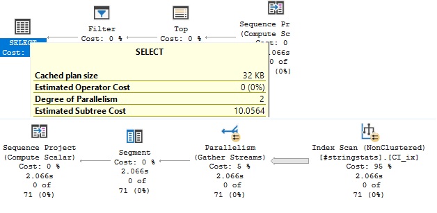
The Index Scan operator to the right employs parallelism. (If you don't get parallelism when you run the query, it may be because you did not adjust cost threshold of parallelism to 5, despite my suggestion in the beginning of the article.)
Simon then applied the pattern with the COLLATE clause from Rudi's query.
SELECT *
FROM  (SELECT  row_number() OVER (ORDER BY CI) r
       FROM    #stringstats
       WHERE   CI LIKE '%xx' COLLATE SQL_Latin1_General_CP1_CI_AI ) d
WHERE r BETWEEN 0 AND 100
The result is baffling:
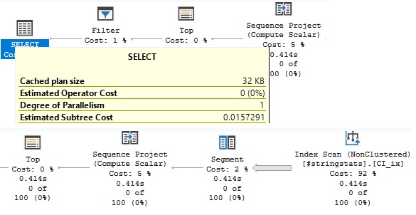
This time there is no parallelism, and if you look at the estimated cost for the query you understand why; it is very low. But that only raises the next question: How could the COLLATE clause have such a huge impact on the costing? When I first saw this I was mighty confounded and the word "bug" may very well have come to my mind. But, as often is the case with SQL Server, there is an explanation and Vassilis Papadimos from the query-processing team was kind to tell us what was going on.
A little known feature in SQL Server is string summary statistics. For a string column, SQL Server tracks the occurrence of substrings in a special place in the statistics blob. This is by no means a new feature, but it has been in the product since SQL 2005. It is one of those features I had heard of but never had looked into, and I had more or less forgotten it. Until Vassilis reminded me.
If you go back to the first plan, you can see that it says 0 of 71 below the Index Scan operator. That is, zero rows were retrieved when 71 was estimated. 71 of one million rows is a very low estimate. Let's look at the estimates in the XML for this operator:
<RelOp AvgRowSize="51" EstimateCPU="0.550079" EstimateIO="9.03646"
EstimateRebinds="0" EstimateRewinds="0" EstimatedExecutionMode="Row"
EstimateRows="70.8215"
EstimatedRowsRead="1000000" LogicalOp="Index Scan" NodeId="5"
Parallel="true" PhysicalOp="Index Scan"
EstimatedTotalSubtreeCost="9.58654" TableCardinality="1000000">
You may note that EstimateRowsWithoutRowGoal is absent, and EstimateCPU+EstimateIO is equal to EstimatedTotalSubtreeCost. That is, there is no row goal here. The optimizer did not find xx in the string summary statistics, so it had no reason to expect very many matches. It still arrived at an estimate of 71 rows. Exactly where this number comes from, I don't know, but I assume that it is some sort of safeguard to cover up for the fact that the string statistics are sampled. (As I understand it, they are always sampled, never based on a full scan.) With an estimate of 71 rows and hundred rows being asked for, the optimizer (correctly) assumes that the query will have to scan the full table. This makes the query expensive enough to warrant the use of parallelism. (When cost threshold for parallelism is set to 5.)
On the other hand, for the second query there is an indication already in the image that there is a row goal: it says 0 of 100. That is, the optimizer expects to find the full 100 rows that were asked for. And if we look at the estimates in the XML, we see this:
<RelOp AvgRowSize="51" EstimateCPU="1.10016" EstimateIO="9.03646"
EstimateRebinds="0" EstimateRewinds="0" EstimatedExecutionMode="Row"
EstimateRows="100" EstimateRowsWithoutRowGoal="90000"
EstimatedRowsRead="1111.11" LogicalOp="Index Scan" NodeId="5"
Parallel="false" PhysicalOp="Index Scan"
EstimatedTotalSubtreeCost="0.0145322" TableCardinality="1000000">
This time, there is an EstimateRowsWithoutRowGoal of 90 000, and the estimated subtree cost is not the sum of the estimated CPU and I/O costs. Why did the COLLATE clause have this effect? A specific answer is that the string statistics are built according to the collation of the column, and what matches in one collation may not match in another. Therefore, the optimizer considers the string statistics to be of no relevance and instead it applies a standard hit rate (or in other words a guess) that happens to be 9 %, which explains that number of 90 000. When only 100 rows are asked for, the optimizer assumes that it will find those imaginary 100 xx rows quickly, applies a row goal and arrives at this low cost to find that there absolutely is no reason for parallelism. So here you see another reason why a row goal can go wrong: there is a bad estimate in the mix.
The real answer is more general: it is the same blues as always. If you entangle a column in an expression that typically precludes an Index Seek. But not only that, it also precludes the use of statistics. Try this query, which logically is exactly the same as the original:
SELECT *
FROM  (SELECT  row_number() OVER (ORDER BY CI) r
       FROM    #stringstats
       WHERE   left(CI, 80) LIKE '%xx') d
WHERE r BETWEEN 0 AND 100
The plan and the cost are the same as for the query with the COLLATE clause.
You may recall that Rudi's query also included an ESCAPE clause. Does the ESCAPE clause also have the same effect? Yes, if you try:
SELECT *
FROM  (SELECT  row_number() OVER (ORDER BY CI) r
       FROM    #stringstats
       WHERE   CI LIKE '%xx' ESCAPE '\') d
WHERE r BETWEEN 0 AND 100
You will find that you get the same "cheap" plan as with the COLLATE clause. The ESCAPE clause is part of the LIKE operator and does not affect the CI column, but since it alters the meaning of the search pattern, the string statistics are no longer applicable. (Well, you could argue that they still are, if somewhat less accurate. But the optimizer discards them entirely anyway.)
I said previously that the statistics could be different depending on the collation. Here is an example to illustrate this. Run these queries:
SELECT COUNT_BIG(*) FROM #stringstats WHERE CI LIKE '%KLMN%'
SELECT COUNT_BIG(*) FROM #stringstats WHERE CS LIKE '%KLMN%'
Below are the query plans I get. (Keep in mind that since data is mostly random, you will get slightly different numbers when you run this yourself.)
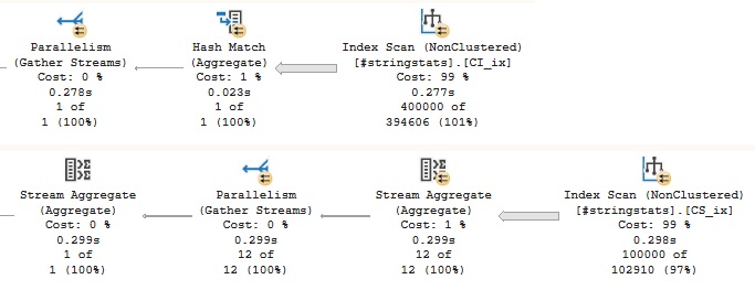
Of main interest here are the Index Scan operators and the actual vs. estimate values. To repeat: When it says 400000 of 394606, this means that the actual number of rows retrieved was 400 000, while the estimated number was 394 606. The estimates are conspicuously close to the actual values for both operators. Note also that the different estimates also result in different operators to implement the COUNT_BIG aggregate.
Here we worked with a search pattern with both leading and trailing wildcards, but the statistics are stored in such a way that the optimizer can handle the special cases that there is only a trailing or leading wildcard. Consider these queries:
SELECT COUNT_BIG(*) FROM #stringstats WHERE CI LIKE 'AA%'
SELECT COUNT_BIG(*) FROM #stringstats WHERE CI LIKE '%AA%'
SELECT COUNT_BIG(*) FROM #stringstats WHERE CI LIKE '%AA'
Here are the rightmost operator for each query:
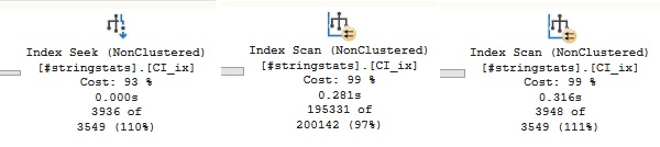
As you can see all three queries have different estimates. You may note that the first query uses an Index Seek, since this is possible in this case. (If the estimate in this case comes from the regular histogram? No, the string summary statistics are used here as well. I will come back to that.)
Here is an example to illustrate how string summary statistics can play a significant role in the choice of query plans. Consider this query in Northgale with its two variations in the condition on Employees.LastName:
SELECT O.OrderID, O.OrderDate, O.CustomerID, C.CustomerName,
       E.FirstName, E.LastName, P.ProductName, OD.Quantity, OD.UnitPrice,
       O.ShipAddress
FROM   Orders O
JOIN   "Order Details" OD ON O.OrderID = OD.OrderID
JOIN   Customers C ON C.CustomerID = O.CustomerID
JOIN   Employees E ON E.EmployeeID = O.EmployeeID
JOIN   Products P ON P.ProductID = OD.ProductID
WHERE  O.RequiredDate > '20011201'
  AND  E.LastName LIKE '%iber%'        -- Matches a single employee with few orders.
--   AND    E.LastName LIKE '%alke%'   -- Matches several employees.
Since these plans are of more size than most other plans in this article, I'm only including low-resolution pictures, but you can still see that the plans have different shapes. The plan to the left is for iber and the plan to the right is for alke.

|

|
In case you don't have Northgale available, you can find the query plans here, if you want to study them more closely. These are text files, but you can download them and change the file type to load them into SSMS or Plan Explorer.
Note: These plans employ features only available in Enterprise Edition. If you run the queries in Standard or Express Edition, you will get plans that are somewhat different from the ones above.
In the examples I have presented so far, I have used literal strings, but in real-life code, it is more likely that the LIKE pattern is supplied in a variable or a parameter. If it is a variable, the value is unknown at compile time, and SQL Server will apply that 9 % guess we saw previously. This example illustrates:
DECLARE @x varchar(80) = '%KLMN%'
SELECT COUNT(*) FROM #stringstats WHERE CI LIKE @x
The estimate is now 90 000, and nowhere close to the actual value of 400 000.
On the other hand, if the value is provided in a parameter, of which the value is known at compile-time, the optimizer will perform its regular sniffing routine to determine the estimate when the query is executed the first time, and then the plan will be reused. For instance, if you run:
DECLARE @sql nvarchar(MAX) = '
SELECT O.OrderID, O.OrderDate, O.CustomerID, C.CustomerName,
          E.FirstName, E.LastName, P.ProductName, OD.Quantity, OD.UnitPrice,
          O.ShipAddress
   FROM   Orders O
   JOIN   "Order Details" OD ON O.OrderID = OD.OrderID
   JOIN   Customers C ON C.CustomerID = O.CustomerID
   JOIN   Employees E ON E.EmployeeID = O.EmployeeID
   JOIN   Products P ON P.ProductID = OD.ProductID
 WHERE    O.RequiredDate > @date
   AND    E.LastName LIKE @str'
EXEC sp_executesql @sql, N'@date date, @str nvarchar(30)', '20011201', '%iber%'
EXEC sp_executesql @sql, N'@date date, @str nvarchar(30)', '20011201', '%alke%'
You will find that the two executions use the same plan. Except that the arrows are thicker in the second execution. And there is a yellow triangle on a Hash Match operator, indicating a spill. A typical example of when parameter sniffing works against us, a problem I discuss in a lot more detail in my article Slow in the Application – Fast in SSMS?.
At this point, the reader may ask how the string summary statistics are stored and how we can view them. The story is that they are utterly unexposed. All there is to see is found in the first result set from DBCC SHOW_STATISTICS. For instance, if you run:
DBCC SHOW_STATISTICS(#stringstats, CI_ix)
You can see this:

YES in the column String Index confirms that there are string summary statistics on this column.
As for the statistics themselves, there is no "civilised" way to inspect them, but you would have to use DBCC PAGE and try to figure out. Or try to decode what comes out of DBCC SHOW_STATISTICS WITH STATS_STREAM (which is explicitly documented as unsupported). And, no, I have not tried this myself. What I have been told is that the statistics are stored in a trie structure. I can't say that I am very familiar with tries myself, but if you want to know more, you can read the article about Tries in Wikipedia.
While string summary statistics may be a feature that many are unacquainted with, there certainly users who are aware of them. One of them is a person using the alias "Hubert" who posted a question on the Microsoft Q&A forum about string-summary statistics and UTF‑8 collations. To show his point, Hubert's post includes repros, but I will use the table we already have:
SELECT COUNT_BIG(*) FROM #stringstats WHERE UTF8 LIKE '%klmn%'
SELECT COUNT_BIG(*) FROM #stringstats WHERE nvarchar LIKE N'%klmn%'
Keep in mind here that both columns have the same collation, but the UTF8 column is varchar and the nvarchar column is of the data type with that name.
When you look at the Index Scan operators in the execution plans, you see something like this:
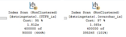
The estimate for the nvarchar column is very accurate, but the estimate for the varchar column is off quite a bit. And if we look at the estimated number, 90 000, it looks very much like that default assumption of a 9 % hit rate. Why is it so? If you run:
DBCC SHOW_STATISTICS(#stringstats, UTF8_ix)
You get the answer:

It says NO in the String Index column. And this is not unique to this particular UTF8 collation, but SQL Server never creates string summary statistics for varchar columns with a UTF‑8 collation. This is described in the topic for DBCC SHOW_STATISTICS for the column String Index. (Which is the only documentation I have been able to find for the feature at all.) So this is apparently a conscious decision. Why, I don't know, but Hubert offered one more observation in his post. Consider these two queries where we are looking for a pattern without a leading %. We are also forcing compatibility level 160 for the queries:
SELECT COUNT_BIG(*) FROM #stringstats WHERE UTF8 LIKE '8D%'
OPTION (USE HINT('QUERY_OPTIMIZER_COMPATIBILITY_LEVEL_160'))
SELECT COUNT_BIG(*) FROM #stringstats WHERE nvarchar LIKE N'8D%'
OPTION (USE HINT('QUERY_OPTIMIZER_COMPATIBILITY_LEVEL_160'))
This is how the Index Seek operators looked in my environment:
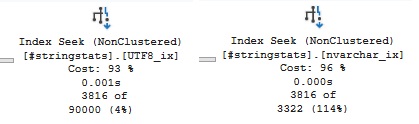
For the UTF8 column, the estimate is obviously the default assumption of 9 %, whereas the estimate for the nvarchar column is decently accurate.
Remove those hints to run the query under compatibility level 170:
SELECT COUNT_BIG(*) FROM #stringstats WHERE UTF8 LIKE '8D%'
SELECT COUNT_BIG(*) FROM #stringstats WHERE nvarchar LIKE N'8D%'
This results in:
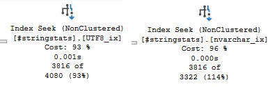
The estimate for the nvarchar column is the same as above, but the estimate for the UTF8 column is now quite close to the mark! Although, if you try other search strings, not all yield equally accurate estimates. I have loaded #stringstats multiple times, but every time the search patterns '8E%' and '8F%' yield estimates that are way lower than the actual values, often only two-digit numbers. (For '8F%' it is often just a single row!) On the other hand for '89%', the estimate is over 450 000 rows. At the same time, estimates for the nvarchar column are quite close to the actual values for any character pair I try. So what is going on?
The change that Microsoft made in SQL 2025 is that in lieu of string summary statistics, for UTF‑8 columns they look at the regular histogram for the column if the search pattern does not have a leading wildcard. If you want to convince yourself of this, you can look at the properties of the Index Seek operator to find this:
Seek Keys[1]: Start: [tempdb].[dbo].[#stringstats].UTF8 >= Scalar Operator('8D');
              End: [tempdb].[dbo].[#stringstats].UTF8 < Scalar Operator('8E')
If you run this query:
SELECT COUNT_BIG(*)
FROM   #stringstats
WHERE  UTF8 >= '8D'
  AND  UTF8 < '8E'
You will find that the estimate is the same as for the LIKE query.
It is quite clear from these examples that when you have a search string without a leading wildcard, so that the histogram is an option at all, the optimizer still prefers the string summary statistics over the histogram. I guess that Microsoft has come to the conclusion that the string statistics generally produce better estimates than the histogram, despite the fact that the string statistics are always sampled. This aligns with some of the examples I mentioned above, and if you play around and try more strings you will see more examples where the estimates from the histogram deviates considerably from the actual values. (The example with '89%' is a bit extreme; this is due to that the Seek Keys property in this case only has a lower bound, but no upper.)
Why are there no string summary statistics for UTF‑8 collations? One possibility is that when they added the UTF‑8 collations in SQL 2019, they ran out of time, and never came around to add the support for string statistics. However, the fact that they made this change in SQL 2025, rather than just adding the missing support, invites speculation that there is some technical challenge that holds them back. What that technical challenge might be, I don't know.
The fact that UTF‑8 collations do not have string summary statistics permits us to get an idea of how much space these tries take up. We can run DBCC SHOW_STATISTICS WITH STATS_STREAM for one of the other columns and the UTF8 column and compare the sizes:
USE tempdb
go
CREATE TABLE #statsstream (id     int IDENTITY   NOT NULL PRIMARY KEY,
                           stream varbinary(MAX) NOT NULL,
                           rows   bigint         NOT NULL,
                           pages  bigint         NOT NULL)

INSERT #statsstream(stream, rows, pages)
   EXEC ('DBCC SHOW_STATISTICS(#stringstats, CI_ix) WITH STATS_STREAM')
INSERT #statsstream(stream, rows, pages)
   EXEC ('DBCC SHOW_STATISTICS(#stringstats, UTF8_ix) WITH STATS_STREAM')

SELECT id, datalength(stream)
FROM   #statsstream
When I run it, the datalength value for CI_ix is 135 866, while it is 16 983 for UTF8_ix. So in this case, the string summary statistics seems to take up a little more than 100 kB.
You may think that for a long column like a nvarchar(MAX), the statistics can grow really huge. But it is not really so, because there is a restriction that I learnt from an old article by David Durant on SQL Server Central. For longer columns, the statistics are built on the first 40 and the last 40 characters in the string and what is in between is ignored. Here is an example to illustrate:
DROP TABLE IF EXISTS #extralong
CREATE TABLE #extralong(str nvarchar(200) COLLATE French_100_CI_AS NOT NULL)
INSERT #extralong (str)
   SELECT concat(space(34),
                 choose(value % 5 + 1, N'Hello', N'Ciao', N'Nihao', N'Serwus', N'Cześć'),
                 space(10), ' Man in the middle ',
                 space(10),
                 choose(value % 5 + 1, N'Shalom', N'Hej', N'Hola', N'Moi', N'Salve'),
                 case when value > 6700 then space(34) end)
   FROM   generate_series(1, 100000)

CREATE STATISTICS str_stat ON #extralong(str) WITH FULLSCAN
go
SELECT COUNT_BIG(*) FROM #extralong WHERE str LIKE '%Ciao%'
SELECT COUNT_BIG(*) FROM #extralong WHERE str LIKE '%middle%'
SELECT COUNT_BIG(*) FROM #extralong WHERE str LIKE '%Hej%'
I get these three Table Scan operators:
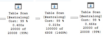
That is, for the words at the beginning and end of the strings, the estimates are very accurate. On the other hand, the estimate is way off for middle, despite that this word appears in all rows. This is due to that it only appears in the trie for the first 6 700 rows where there is no final padding of 34 spaces. For the rest of the rows, middle is in this "dark zone" between the 40 first and the 40 last characters.
The string summary statistics are subject to automatic updates just like normal statistics, as illustrated by this example:
UPDATE #stringstats
SET    CI = replace(CI, '1234klmn', '1234spqr')
WHERE  CI LIKE '%1234klmn%'
go
SELECT COUNT_BIG(*) FROM #stringstats WHERE CI LIKE '%klmn%'
When I run it, the text below the Index Scan operator says 300000 of 304544. (Compare that to the estimate we had earlier.)
Finally, you may ask if these statistics are also used for regular expressions, introduced in SQL 2025, but the answer is no. Consider:
SELECT COUNT_BIG(*) FROM #stringstats WHERE regexp_like(CS, 'klmn')
The estimate is 90 000 which looks very much like that standard assumption of 9 %. And it is not really surprising. As we have seen, string summary statistics are collation-dependent, but regular expressions are not collation-aware. (Essentially, they are binary, although there is a flag to request them to be case-insensitive.)
Before we draw this to a close, I'd like to go back and revisit Rudi's query that we started with, because there are a few observations that I left out to keep focus on the main points, but that still are interesting to make.
When Rudi posted his question, he remarked that the query included some anti-patterns, and one was the use of row_number for the pagination rather than OFFSET FETCH. As the thread progressed, and Hugo showed him that there was a Top operator and a row goal, his concern about row_number seemed to wane. However, as we shall see in this section, his initial comment was not entirely unfounded.
Here are four queries to retrieve 500 rows from our #stringstats table, one using TOP, one using OFFSET FETCH, one using TOP with 500 in a local variable, and one using the pattern with row_number:
SELECT TOP (500) CI
FROM    #stringstats
WHERE   CI LIKE '%KLMN%'
ORDER   BY CI

SELECT CI
FROM   #stringstats
WHERE  CI LIKE '%KLMN%'
ORDER  BY CI
OFFSET 0 ROWS
FETCH FIRST 500 ROWS ONLY

DECLARE @rows int = 500
SELECT  TOP(@rows) CI
FROM    #stringstats
WHERE   CI LIKE '%KLMN%'
ORDER   BY CI

SELECT CI
FROM  (SELECT  *, row_number() OVER (ORDER BY CI) r
       FROM    #stringstats
       WHERE   CI LIKE '%KLMN%') d
WHERE r BETWEEN 0 AND 500
Here are execution plans (with the final SELECT operator left out for space reasons):
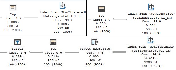
There are only three plans, because the first two queries generate identical plans, at least graphically. This is the plan to the left in the upper row. There is a Top and an Index Scan operator, and that's all. Furthermore, the estimates are correct. (500 of 500.) The plan to the right is the query with the variable. Here the estimates for the operators are 100 rows. Since the value of the variable is not known at compile time, the optimizer applies a default guess, which seems to be 100 rows.
In the bottom row, we have the plan for the row_number query. As you can see, it includes two more operators, so that we have Filter, Top, Window Aggregate and Index Scan in that order. We can see that for the Index Scan operator, both the actual and estimated number of rows is different from the first two queries. The fact that the Windows Aggregate and Index Scan operator processes more than the requested 500 rows seems to be due to that these operators run in batch mode. And indeed, when I run the query on Standard Developer Edition, the Index Scan operator only reads 500 rows. The estimates are always 100, no matter the edition. That seems like this default assumption when the optimizer does not know the value at compile time. But why?
As Rudi pointed out to me, the answer is found if you hover over the Top operator. At the bottom of the popup, you can see this:

This CASE expression looks a little wild, but I guess it is a general transformation that works also if the values for the row_number filter are variables or more complex expressions. In any case, it seems that the optimizer is not able to compute this expression at compile-time, so it has to fall back on the default assumption. (The optimizer is able to compute values of some expressions in certain contexts, but this is apparently not such a case.)
As you can see, using the pattern with row_number over OFFSET FETCH (or TOP) comes with two issues, although none of them should be overplayed:
In the main chapter on row goals, I made it seem that the Id column is numeric and monotonically growing, and this was also my assumption when I wrote the first outline of the article. But at one point I looked at the execution plan that Rudi had shared and paid attention to the actual query text, which made it clear that my assumption was incorrect. To wit, the part that in Rudi's anonymised version read:
T0.varchar1 LIKE 'something%' ESCAPE '\'
            COLLATE SQL_Latin1_General_CP1_CI_AI
does in fact read:
[T0].[Id] LIKE 'vb%' ESCAPE '\' COLLATE SQL_Latin1_General_CP1_CI_AI
So Id is actually a string! Exactly what this vb is, I don't know, but my guess is that it is a prefix of some sort. Whatever, this means that there is no particular reason to assume a correlation between Id and ModifiedDate. Despite this revelation, I decided to keep the story that I had, because tables with monotonically growing ids are very common, and in such tables you can expect more than one column to have a correlation of some sort with the id. For instance, consider a PayStatus column in a table with ten years worth of orders. All rows with the value Unpaid are likely to be among the orders from the current year. (Older orders that were never paid are likely to have been changed to WrittenOff or similar.) One more example is a query that looks for orders for an employee who joined the company fairly recently.
Nevertheless, I find it be interesting to discuss what were the real causes of why Rudi's query was costed so low, preventing the use of parallelism, and I have identified three, and the first one was the use of row_number over OFFSET FETCH. Before I go on to look at the second and third reasons, here are some key numbers, of which some have appeared earlier in the article, and some have not:
Also, a reminder of the two LIKE conditions in the query, with one more detail of the actual query revealed, to show that vb reappears in the second search pattern as well:
AND (T0.Id LIKE 'vb%' ESCAPE '\' COLLATE SQL_Latin1_General_CP1_CI_AI
  OR T0.varchar2 LIKE '%vb%' ESCAPE '\' COLLATE SQL_Latin1_General_CP1_CI_AI)
Could this have any bearing to why the cost for the CI Scan in Rudi's was underestimated? That does not seem unlikely. I have very little idea what this varchar2 might be, but my speculation is that it is a rare thing that rows have vb in this column when Id starts with something else. And specifically, there are less than 200 of them. Thus, if my speculation is correct, to find 200 matching rows in total, the scan has to find one or rows where Id starts with vb. Given the alphabet, these rows are likely to be located towards the end of the clustered index. The fact that the query had to read all but 18 225 rows from the table aligns with this assumption.
The third reason why the CI Scan was underestimated is something we learnt in the previous chapter: Those COLLATE and ESCAPE clauses prevent the optimizer from using the string summary statistics and therefore it has to resort to making blind guesses. Instead of an estimate around 8 000 rows, the optimizer comes up with a much higher value. Now, the observant reader will note that there is something that does not match up. The value for EstimateRowsWithoutRowGoal is about one third of the number of rows in the table, which is way higher than what two blind estimates of 9 % added together could give. I scratched my head for a while, but eventually I found this in the plan XML:
CardinalityEstimationModelVersion="70"
That is, the database is configured to use the legacy cardinality estimator, which indeed has different rules for this situation. First run these queries and observe the estimates for the Index Scan operators:
SELECT COUNT_BIG(*) FROM #stringstats
WHERE CI LIKE '%1234ABCD%' ESCAPE '\' COLLATE SQL_Latin1_General_CP1_CI_AI

SELECT COUNT_BIG(*) FROM #stringstats
WHERE CI LIKE '%34AB%' ESCAPE '\' COLLATE SQL_Latin1_General_CP1_CI_AI

SELECT COUNT_BIG(*) FROM #stringstats
WHERE CI LIKE '%4A%' ESCAPE '\' COLLATE SQL_Latin1_General_CP1_CI_AI
The estimate is 90 000 rows in all three cases.
Now run the queries with the legacy cardinality estimator:
SELECT COUNT_BIG(*) FROM #stringstats
WHERE CI LIKE '%1234ABCD%' ESCAPE '\' COLLATE SQL_Latin1_General_CP1_CI_AI
OPTION (USE HINT('FORCE_LEGACY_CARDINALITY_ESTIMATION'))

SELECT COUNT_BIG(*) FROM #stringstats
WHERE CI LIKE '%34AB%' ESCAPE '\' COLLATE SQL_Latin1_General_CP1_CI_AI
OPTION (USE HINT('FORCE_LEGACY_CARDINALITY_ESTIMATION'))

SELECT COUNT_BIG(*) FROM #stringstats
WHERE CI LIKE '%4A%' ESCAPE '\' COLLATE SQL_Latin1_General_CP1_CI_AI
OPTION (USE HINT('FORCE_LEGACY_CARDINALITY_ESTIMATION'))
The estimates are, in order: 83 000, 166 000 and 331 999. Thus, with the legacy cardinality estimator, the default assumption is more "sophisticated" and the length of the pattern is taken into consideration. Furthermore, when I run some more tests, it seems that the legacy estimator also considers the length of the string column. Searching for the pattern '%1234ABCD%' in a varchar(160) column, I get a default assumption of 98 596, higher than what I got above.
I can't deny that the idea as such makes sense. The longer the search string, the smaller the likelihood for a match. And the longer the column, the better the chances for a match. But it seems that the base values the legacy estimator works from are just way too high. How likely is it that an eight-character long string will yield a hit rate of 8-10 %? Or that a two-character long string will appear in 40 % of the rows?
In any case, these wild default assumptions explain why EstimateRowsWithoutRowGoal was so high in Rudi's query.
I should add that when the string-summary statistics can be used, I get the same estimates with the legacy cardinality estimator as with the modern estimator.
So these were the three reasons why Rudi's query was underestimated:
Of these three reasons, which contributed most to Rudi's performance problem? While the third reason leads to an error for EstimateRowsWithoutRowGoal that is spectacular, I would say that it is still the second issue that is the main problem. Let's say that it would actually be in Rudi's powers to edit the query and remove those COLLATE and ESCAPE clauses, and while he was at it he would also apply OFFSET FETCH. The optimizer would still see fit to apply a row goal, and it would still assume a uniform distribution, despite that the matching rows are all close to the end of the clustered index. It would be less optimistic how quickly it would find the rows, and therefore assign the CI Scan operator a higher cost. I don't know the formula that the optimizer uses to scale the cost when applying a row goal, but as a simple calculation, let's scale the estimated cost with the ratio between the bad estimate and the actual number of rows, and also adjust for the corrected row goal:
SELECT 2 * 0.16493 * 329146/8000
This returns 13.6. That is, yes, with the default setting for cost threshold for parallelism, Rudi would have gotten the parallelism he desired. But he would not, if the setting had been adjusted to conform to modern "best practice". (See rant in the beginning of the article.)
So in the end, the main problem was the location of vb in the alphabet. But the bad estimates due to hiding the columns in expressions certainly help to make matters worse. And the final insult to injury was the use of row_number instead of OFFSET FETCH.
The solution Rudi eventually arrived at was to add a Query Store hint to inject DISABLE_OPTIMIZER_ROWGOAL. And this hint can often be the way out when correlation causes the optimizer to be too optimistic about the effect of a row goal. But keep in mind that this hint is not always the solution. Remember the example where we looked for the most recent order for each employee. Here we got better results by adding an index hint.
I'd like to extend thanks to Data Platform MVP Rudi Bruchez for presenting this interesting problem, to my fellow Data Platform MVPs Hugo Kornelis and Simon Sabin for an interesting discussion, to Vassilis Papadimos for making me finally understand the impact of string summary statistics. Rudi and Hugo were also both kind to make corrections and add further observations to my original draft. I also like to thank "Hubert" for raising the point about UTF‑8 collations. Not only was the point interesting as such, but it was also his post that finally sparked me to write this article that had been on my mind for over a year. And thanks to Paul White for writing those articles on row goals (and many other articles about optimizer internals).
As always, I welcome comments to my articles, so if you feel that you have something to add or you have spotted an error, please mail me on esquel@sommarskog.se. And that very much includes pointing out spelling or grammar errors that you find! Since I am not writing for a publisher, I will have to rely on my readers for the proof-reading.
This article is now at the end. You have read about row goals and string summary statistics, and maybe you have learnt a few things you did not know previously. I hope that you have found it enjoyable and informative.